Cloud cost management

TL;DR — Compute is usually the largest line item on your cloud bill. Bills tell you what you spent, not what you used. Measure utilisation with percentiles (P95/P99), not averages. Prefer always-on elastic infrastructure over scheduled shutdowns, and let Kubernetes bin-pack workloads to squeeze more value out of every node.
Back in 2015, public cloud services were not well understood. Large enterprises debated whether migrating to the cloud would meet their security requirements, paralysed by fear of the unknown. We have come a long way since — digital transformation is now synonymous with cloud migration. The benefits of on-demand infrastructure and elasticity have made engineers more productive and businesses happier with the promise of improved time-to-market.
Note: A key assumption in this write-up is that your organisation has a considerable portion of applications that are stateless and can be horizontally scaled to make the most of cloud infrastructure. I will address optimising cost for other workload types in a follow-up post.
Elasticity — the double-edged sword
Public cloud is a double-edged sword, especially when it comes to on-demand infrastructure and elasticity. Although spinning resources up and scaling out horizontally takes little effort, gracefully shutting down and draining connections to those same resources requires more foresight and engineering rigour. Get this wrong and you could rack up a hefty bill.
The pay-as-you-go model is not as straightforward as it sounds either. Several services have a complex billing model where data retrieval is charged at a different rate than data storage on the same service. AWS X-Ray is a good example. When X-Ray is used together with services such as AWS API Gateway and Lambda in a single solution, forecasting spend gets considerably more complex.
Focusing on compute as a starting point
I have had the privilege of working with several clients, large and small, across domains ranging from finance and utilities to gaming. I see the nuances of how their teams grow and adopt different technologies on the road to cloud adoption. Despite domain differences, there are always similarities in how they consume resources.
Compute is generally the largest cloud cost. The figure below shows the usage cost by service for four companies across different domains. In every case, compute is the biggest component, contributing between 40% and 70% of the bill.
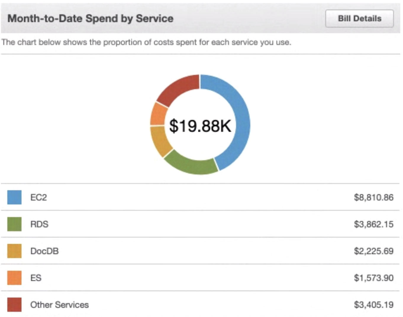
Compute (EC2) consistently dominates the cloud bill across organisations.
Understanding the cost-to-usage ratio
Public cloud vendors do a good job of breaking down spend by line item and showing billing trends. What they do not do well is highlight the actual usage of each service. For example, the EC2 line item below shows how much I am paying — but not how much of that capacity is actually being used.
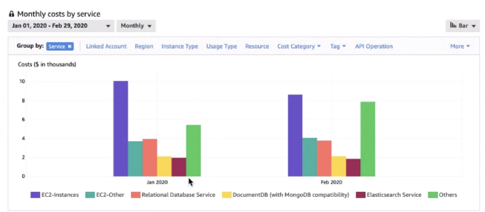
Bills tell you what you spent, not what you used.
You need to dig deeper to understand utilisation. Amazon CloudWatch on AWS and Google Cloud’s operations suite (formerly Stackdriver) on GCP do a reasonable job of this, and both AWS Compute Optimizer and the GCP Recommender now provide right-sizing suggestions out of the box.
Leveraging the right data for informed insights
What you cannot measure, you cannot optimise — and measuring the right metrics matters even more. To explore inefficiencies in compute utilisation, start by collecting CPU and RAM metrics. CloudWatch makes plotting CPU usage straightforward.
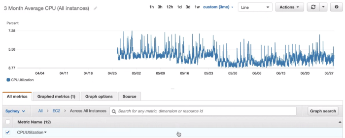
Average CPU utilisation over three months — looks idle.
Averages are misleading. Over a long window, averages mask sustained CPU spikes. The graph above shows an average CPU utilisation of around 7%. The same dataset looks quite different at the P95 and P99.
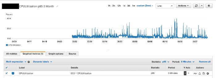
P95 CPU utilisation over the same period — closer to the truth.
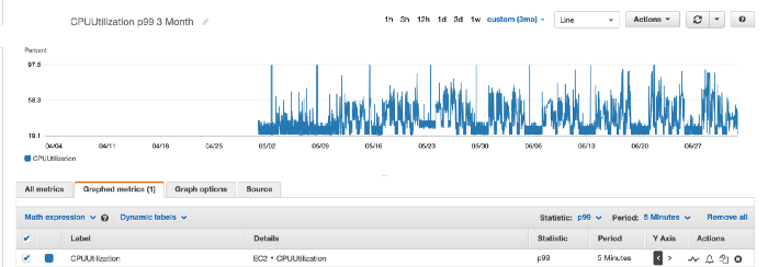
P99 CPU utilisation — what your busiest moments actually look like.
Use percentiles instead. The two images above show CPU utilisation around 16% and 22% at the 95th and 99th percentiles respectively — significantly higher than the average. These measurements paint a far more accurate picture of CPU load and the compute capacity you actually need. A reasonable starting point is to align your autoscaler’s desired state to roughly the P95, Min to the average, and Max with headroom above P99 to absorb genuine bursts.
The same approach applies to RAM. Most cloud providers do not surface memory metrics out of the box because the hypervisor cannot see inside the guest. On AWS, the CloudWatch Agent is the supported way to collect memory and disk metrics from EC2.
Always-on elastic infrastructure is the future
It is common practice for organisations to turn off non-production infrastructure overnight or over the weekend. With more teams now distributed across timezones, scheduled shutdowns are not always feasible.
It is also worth asking how often you have walked into work on a Monday morning to find that not all of your infrastructure has booted as expected. Teams that move fast tend to update their infrastructure-as-code often and encounter issues more frequently. Broken infrastructure drains productivity, which is another argument for leveraging elasticity rather than turning resources off entirely. In our experience, the productivity loss from infrastructure issues often outweighs the savings from weekend shutdowns.
An always-on approach lets teams work across timezones and flexible hours. Kubernetes can scale a cluster from hundreds of nodes down to a handful without manual intervention. Resource allocation for every container can be adjusted in seconds with a single API call.
Setting requests and limits before you bin-pack
Sizing a Kubernetes workload comes down to two values per container: requests (the floor the scheduler guarantees) and limits (the ceiling the kernel enforces). The percentile work above feeds directly into these — set requests close to your P95 so the scheduler has enough information to pack effectively, and set limits with headroom above P99 to absorb bursts without throttling.
Understanding the power of Kubernetes bin packing
Once you understand the compute requirements of your workload, you need a platform that lets you optimise how those workloads are placed onto your servers. This is where Kubernetes — and its bin-packing scheduler — comes in.

Kubernetes bin packing: like Tetris, but for your workloads.
Bin packing works much like Tetris. Think of each piece as an application workload. Kubernetes takes these container workloads and places them on the same node to maximise resource utilisation. The security, resource sharing and isolation of these containers are also managed by Kubernetes — but that is a topic for another post.
Kubernetes lets you treat compute (CPU and RAM) as a pool rather than a collection of individual servers. This shift in perspective lets you reason about compute requirements across the whole organisation and hand the divvying-up of those resources to the scheduler.
Going further: spot capacity, savings plans, and FinOps
Right-sizing and bin-packing get you a long way, but the next levers worth pulling are pricing-based:
- Spot / preemptible instances for stateless, fault-tolerant workloads can cut compute cost by 60–90%. Tools like Karpenter on AWS and GKE Autopilot on GCP make spot adoption far less painful than it used to be.
- Savings Plans / Committed Use Discounts reward predictable baseline usage with substantial discounts in exchange for a 1- or 3-year commitment.
- FinOps as a practice. The FinOps Foundation framework gives finance, engineering and product a shared language and operating model for managing cloud spend. If cost management is becoming a recurring conversation, formalising it as FinOps is usually the right next step.
Key takeaways
- Start with compute — it is almost always the biggest line item.
- Measure utilisation, not just spend. Bills are not a substitute for telemetry.
- Use percentiles (P95/P99) rather than averages when sizing.
- Set Kubernetes
requestsnear P95 andlimitsabove P99. - Prefer always-on elastic infrastructure over scheduled shutdowns.
- Layer pricing tools (spot, savings plans) on top of a healthy utilisation baseline.
I will dig deeper into stateful workloads, cluster autoscaling strategies and FinOps tooling in upcoming posts.